Extended abstract · accepted as a poster at COMPLEX NETWORKS 2026 · Granada, 2–4 December 2026
Disperse to ignite, concentrate to endure: a decay-driven crossover in modular complex contagions
Synthetic data Every result on this page comes from an uncalibrated simulation: synthetic organisations and, in one robustness check, a real network topology with synthetic behaviour. It describes how the model behaves; it is not a forecast for any real organisation.
In brief
In simulated organisations, dispersing the first adopters spreads a practice further; concentrating them sustains it when people often drop practices that their colleagues do not use.
- In the headline scenario (mean threshold 0.30, 100 seeds) and without relapse, random (dispersed) seeding reaches 72.0% terminal adoption, against 32.4% for whole-team (cluster) seeding: a paired difference of +39.7 pp [35.4, 43.9].
- With relapse, the advantage shrinks and changes sign between the tested rates. When retention requires full reinforcement (r = 1), it falls from +8.4 pp at relapse probability ρ = 0.10 to −5.3 pp at ρ = 0.25 and −11.4 pp at ρ = 0.40.
- In the harshest tested setting, clustered adoption barely moves (32.4% to 29.3%) while dispersed adoption collapses (72.0% to 17.9%).
Brackets give 95% confidence intervals; pp means percentage points. The model is synthetic and uncalibrated, and the crossover was measured in a single organisational setting.
Key terms (seed, terminal adoption, relapse…)
- Seed
- One of the first adopters, chosen by a seeding strategy. Seeds adopt at the start, then follow the same rules as everyone else.
- Terminal adoption
- Adopters as a share of all people when a run ends: at an absorbing state (no one can adopt and no adopter is below the retention bar) or after 100 steps. This is the main measure.
- Cumulative reach
- The share of people who have adopted by a given time. A secondary, descriptive measure.
- Retention
- The share of ever-adopters who remain adopters.
- Relapse probability ρ
- The probability, per step, that an adopter drops the practice while their exposure is below r times their threshold. Relapse is off (ρ = 0) unless stated.
- r
- How much reinforcement retention requires: r = 1 means full reinforcement, r = 0.5 a weaker coupling.
- Paired difference
- Random minus cluster, computed within each organisation: every strategy runs on the same organisations, with the same random numbers for agent selection.
- pp
- Percentage points. The practical band of ±2 pp corresponds to about 40 people.
- “Equivalent”
- Within ±2 pp according to an equivalence test (TOST), for the tested cells and this model only.
Figure 1
 (open the full-resolution image)
How to read it
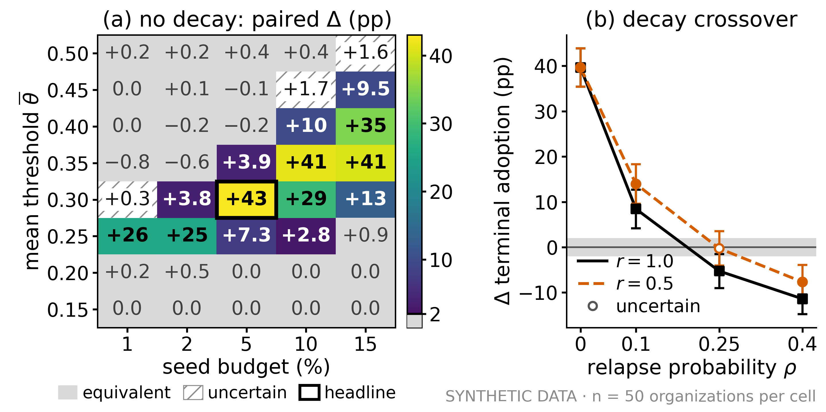
In panel (a), each cell compares random and cluster seeding on the same 50 organisations, for one mean threshold (rows) and one seed budget (columns); the number is the paired difference in percentage points. Coloured cells are wins for dispersion, grey cells are equivalent within ±2 pp and hatched cells are uncertain. The wins form a diagonal “ignition band” that moves to larger budgets as the threshold rises.
The boxed cell is the headline setting, re-run on an independent paired sample: it sits at the top of the band, at +42.6 pp (printed as +43). The headline estimate quoted in the text, +39.7 pp [35.4, 43.9], comes from the main run.
Panel (b) follows the same difference at the headline setting as the relapse probability ρ grows, for r = 1 (black squares) and r = 0.5 (orange circles, dashed line). Points below zero mean that, on average, cluster seeding ends with more adopters; the grey band marks the ±2 pp practical margin.
Text description of Figure 1
Panel (a), titled “no decay: paired Δ (pp)”, is a grid of 40 cells: mean thresholds in rows, seed budgets in columns. Wins for dispersion (14 cells) lie on a diagonal band running from small budgets at low thresholds to large budgets at higher thresholds, with values from +2.8 to +42.6 pp. Equivalent cells (23) lie on both sides of the band: below it, where adoption saturates, and above it, where high thresholds and small budgets starve it. Three cells are uncertain (hatched). No cell shows a detected cluster advantage of practical interest; the largest observed cluster edge is 0.8 pp.
Panel (b), titled “decay crossover”, plots the difference in terminal adoption against the relapse probability ρ, with a grey band marking ±2 pp around zero. Both curves start from the headline difference without relapse. For r = 1, the difference falls to +8.4 pp at ρ = 0.10, −5.3 pp at ρ = 0.25 and −11.4 pp at ρ = 0.40. For r = 0.5, the curve stays higher: its marker at ρ = 0.25 is hollow (uncertain), and it falls below the band only at ρ = 0.40, at −7.7 pp. The figure carries the stamp “SYNTHETIC DATA · n = 50 organizations per cell”.
The question
Getting the staff of an organisation to adopt a new habit is a practical management question. When an organisation wants to spread a costly practice (a tool such as an AI assistant, a work habit), should it concentrate the first adopters, the seeds, in a few dense teams, or disperse them across teams?
A complex contagion does not occur on a single exposure: threshold models need multiple exposures and reinforcement [4]. Cascades on random graphs obey a cascade condition [12], and complex contagions require wide bridges of overlapping ties, which long-range shortcuts destroy [2], [1]. Intervention taxonomies emphasise matching interventions to their context [10]. The expectation that clustered seeding should win comes from the wide-bridges results, obtained largely in populations not already embedded in cohesive groups.
Other results challenge this idea: modularity aids cascades only up to a point [7]; dispersed neighbour seeding outperforms clustered seeding in threshold models [8]; multiple spreaders perform best when placed apart [6]; and random ties outperform clustered ties unless interest wanes quickly [11], [9]. Where these last studies vary the tie structure, this study varies only where the seeds are placed, and asks whether decay, with adopters relapsing, reverses the ordering.
Real organisations are modular: almost everyone belongs to a small, dense team. So what does clustered seeding add when every seed is already surrounded by a cluster?
Results
Synthetic data; unless stated otherwise, 50 paired organisations per condition; brackets give 95% confidence intervals.
Without relapse, dispersed seeding ends with more adopters
In the headline scenario (mean threshold 0.30, 100 seeds), random seeding reaches a terminal adoption of 72.0% ± 9.2% (mean ± SD), against 32.4% ± 11.0% for cluster seeding: a paired difference of +39.7 pp [35.4, 43.9]. On average, random seeding already places seeds in 82 of the 249 line teams; cluster seeding places them in 13.
Across 40 settings: 14 wins for dispersion, 23 equivalent, 3 uncertain
Across 40 combinations of mean threshold and seed budget (Figure 1a), dispersion dominates in 14 cells, along a diagonal ignition band ranging from +2.8 to +42.6 pp (the top value is the boxed headline cell, an independent paired sample). In 23 cells the strategies are equivalent within ±2 pp: saturation at low thresholds, starvation at high thresholds with small budgets. Three cells are uncertain. No cell shows a detected cluster advantage of practical interest (≥ 2 pp); the largest observed cluster edge is 0.8 pp.
With relapse, the advantage shrinks, then reverses
As relapse becomes more likely, the dispersion advantage decreases monotonically in ρ and changes sign between the tested values (Figure 1b). When retention requires full reinforcement (r = 1), the paired difference falls from +8.4 pp [4.2, 12.7] at ρ = 0.10 to −5.3 pp [−9.0, −1.5] at ρ = 0.25 and −11.4 pp [−14.8, −8.0] at ρ = 0.40. With weaker coupling (r = 0.5), the reversal appears only at the highest tested rate: −7.7 pp [−11.5, −3.9] at ρ = 0.40. All runs at ρ ≥ 0.25 ended in absorbing states, which rules out a horizon artefact.
| Seeding | No relapse | r = 1, ρ = 0.40 |
|---|---|---|
| Cluster (whole teams) | 32.4% | 29.3% |
| Random (dispersed) | 72.0% | 17.9% |
Behind the reversal: mainly retention
At r = 1 and ρ = 0.25, the terminal contrast has reversed, while the contrast in cumulative reach (secondary, descriptive) remains inconclusive: −1.8 pp [−5.4, +1.8]. The cumulative-reach contrast is clearly negative only at ρ = 0.40: −7.4 pp [−10.7, −4.1]. The terminal reversal is therefore driven mainly by differential retention, the share of ever-adopters who remain adopters: 0.99 for cluster against 0.86 for random seeding.
Other strategies and the no-seed baseline
Spreading seeds one per team (one-per-team, round-robin coverage) shows no clear difference from random seeding: −1.4 pp [−5.0, +2.2]. Targeting the people with the most informal ties (champions) adds about +3.9 pp over random seeding (descriptive; CI [0.6, 7.1]). A broadcast with no seeds reaches a terminal adoption of 5.5% ± 3.4%, and 0.0% in the 12 tests without innovators (independent panel).
Robustness: other organisations and a real topology
Varying one parameter at a time (organisation size 500, 2,000 or 8,000; team size 5 or 12; silo 0.5, 0.7 or 0.95), the paired difference ranged from +14.7 to +48.3 pp, and no confidence interval crossed zero. These variants were tested without relapse; the crossover was measured in a single organisational setting.
On the real email-Eu-core topology (986 nodes, 42 ground-truth departments, all behavioural attributes synthetic), random seeding exceeds cluster seeding by +13.5 pp [1.0, 26.0] on average over 50 paired attribute draws. Adoption there is bimodal: a low mode (median 9%) and a high mode (median 85%). This replicates the sign, without relapse, on a real modular topology; it is not an empirical validation of the mechanism.
Why it happens in the model
A random seed is usually alone in its team. It starts far below its threshold and, under relapse, may drop the practice immediately. A fully seeded team can keep its members well above their thresholds: a team seeded together can sustain adoption, while a lone seed lacks this support. Dispersed seeding must then activate teams before its seeds relapse, which becomes harder as ρ increases. In this model, the strategy most efficient for spreading a practice is thus not necessarily the most efficient for maintaining it.
This explanation is incomplete. A local predictor of team ignition, pre-specified in the same decision log, failed its validation criterion (AUC 0.64, against a criterion of 0.70) and does not sufficiently explain dispersed activation. Team-level trajectories remain for future work.
Method in plain terms
Organisations. A generator builds two-tier organisations: a formal hierarchy of 2,000 people in eight departments and 249 line teams of eight people on average, plus an informal influence network. Teammates are almost all connected (p = 0.9); each person has about six ties to other teams of the same department, mostly adjacent “sister” teams, and about 0.45 to other departments (silo = 0.85), plus sparse random ties. The structure resembles a nested stochastic block model.
People. Each agent has a personal threshold drawn from a Beta distribution with mean μ = 0.30 and concentration κ = 20; with probability 0.025, an agent is an innovator with a threshold of zero. Exposure is the credibility-weighted share of contacts who had adopted at the previous step. Credibility is 1.0 for close cooperation partners, 0.7 for managers, 0.6 for distant peers and 0.3 for communication partners. Adoption requires being ready (exposure at or above the threshold, and above zero), willing (probability 0.85, drawn once at the start) and able (1.0 here) [3].
Relapse. As long as an adopter’s exposure is below r times their threshold, they drop the practice with probability ρ per step. Relapsed agents may adopt again. Relapse is off unless stated.
Strategies. Four seeding rules, each with a budget of 100 seeds: random; champions (highest informal degree); cluster (whole teams); one-per-team (round-robin coverage). Seeds adopt at the start regardless of readiness and willingness, then follow the same rules as everyone else. A broadcast without seeds serves as the baseline. These are rules fixed in advance, with no claim of optimality [5], [8].
Measures. Terminal adoption (main): adopters as a share of all people when a run ends, at an absorbing state or after 100 steps. Cumulative reach (secondary): the share of people who have adopted by a given time.
Comparisons. In each condition, every strategy runs on the same 50 newly generated organisations, with the same random numbers for agent selection, so contrasts are paired differences within organisations. Pairing is used to control confounding, not for precision.
The model in equations (formula and parameters)
Thresholds: , with μ = 0.30 and κ = 20.
Exposure of agent i at step t:
N(i) is the contact set of i, wi,j the weight (credibility) of j for i, aj the adoption of j at the previous step, and b(t) a communication term used only in the broadcast baseline (0.3 in its first step, 0 thereafter).
An agent is ready when its exposure is at or above its threshold and above zero. An adopter whose exposure is below r times its threshold relapses with probability ρ per step.
| Parameter | Value |
|---|---|
| People, departments, line teams | 2,000; 8; 249 |
| Within-team tie probability p | 0.9 |
| Ties to other teams of the same department | about 6 per person |
| Ties to other departments | about 0.45 per person (silo = 0.85) |
| Threshold distribution | Beta, μ = 0.30 (headline value; the mean threshold is varied in Figure 1a), κ = 20 |
| Innovator probability | 0.025 |
| Credibility weights | 1.0 (close cooperation), 0.7 (managers), 0.6 (distant peers), 0.3 (communication) |
| Willing | probability 0.85, drawn once |
| Able | 1.0 |
| Broadcast term b(t) | 0.3 in the first step, then 0 |
| Seeds per strategy | 100 (headline value; the seed budget is varied in Figure 1a) |
| Run length | until an absorbing state, at most 100 steps |
| Organisations per cell | 50, paired across strategies |
Statistical protocol (pairing, tests, verdicts)
The two confirmatory families, the regime map (Figure 1a) and the decay grid (Figure 1b), were pre-specified in the decision log after an exploratory panel (n = 12 organisations per cell, not used in Figure 1). Within each family, Holm correction was applied to the difference tests and to the TOST equivalence tests against a practical band of ±2 percentage points (≈ 40 people). Each cell receives one of three verdicts: “win”, “equivalent” (within ±2 pp, for the tested cells and model) or “uncertain”. Random-number seeds were frozen before execution.
The champions contrast and the cumulative-reach contrasts are descriptive.
What this work does not show
- A model, not a measurement. All of this holds within an uncalibrated synthetic model: thresholds are unobserved, decay parameters are set on a grid, and time is abstract.
- One setting for the crossover. The reversal under relapse was measured in a single organisational setting; the organisational variants were tested without relapse.
- A bracketed sign change. The sign changes between tested values of ρ: for r = 1, the difference is still positive at ρ = 0.10 and already negative at ρ = 0.25. Where exactly it changes is not estimated.
- Terminal adoption, the main measure. The reversal is observed on terminal adoption. At r = 1 and ρ = 0.25, the contrast in cumulative reach (secondary, descriptive) is inconclusive; it is clearly negative only at ρ = 0.40.
- A real topology, synthetic behaviour. The email-Eu-core result replicates the sign on a real topology, without relapse and with synthetic behavioural attributes. It is not an empirical validation of the mechanism.
- An incomplete mechanism. The pre-specified local predictor of team ignition failed its validation criterion.
- A narrow equivalence. “Equivalent” holds for the tested cells and this model only.
- Fixed rules. The four strategies are rules fixed in advance, with no claim of optimality.
- Not advice. Nothing here is a recommendation for real organisations.
Read, reproduce, cite
Read
The extended abstract: PDF, 4 pages, 346 kB. This is the camera-ready version, dated 5 October 2026.
SHA-256 of the file: 75a549635f15579a03255de7ad9b19beb2cb6b3dd77f19070f123dbdff72b993
Reproduce
Code, decision log (D1–D23) and reproduction pipeline: github.com/PaulBufort/adoption-sim, under the AGPL-3.0 licence. Every reported estimate is machine-extracted from the versioned results and checked by an audit script. The decision log itself: docs/decisions.md.
Cite
Bufort, P.: Disperse to ignite, concentrate to endure: a decay-driven crossover in modular complex contagions. Extended abstract, COMPLEX NETWORKS 2026, 15th International Conference on Complex Networks and Their Applications, Granada, Spain (2026).
@inproceedings{bufort2026disperse,
  author    = {Bufort, Paul},
  title     = {Disperse to ignite, concentrate to endure: a decay-driven
               crossover in modular complex contagions},
  booktitle = {Book of Abstracts of the 15th International Conference on
               Complex Networks and Their Applications (COMPLEX NETWORKS 2026)},
  address   = {Granada, Spain},
  year      = {2026},
  note      = {Extended abstract},
  url       = {https://paulbufort.com/cn2026/}
}
The ISBN and page numbers will be added when the Book of Abstracts is published.
Granada, December 2026
This extended abstract was accepted at COMPLEX NETWORKS 2026, the 15th International Conference on Complex Networks and Their Applications, held at the University of Granada (UGR) on the Fuentenueva campus. Tutorials take place on 1 December and the main conference runs on 2–4 December 2026. It will be presented as a poster; the poster session will be announced here once the programme is published.
If you are attending and would like to discuss the model (the relapse rule, the threshold distribution, the organisational topology), come to the poster or write to me at contact@paulbufort.com.
References
- [1]Centola, D.: The spread of behavior in an online social network experiment. Science 329(5996), 1194–1197 (2010). doi:10.1126/science.1185231
- [2]Centola, D., Macy, M.: Complex contagions and the weakness of long ties. Am. J. Sociol. 113(3), 702–734 (2007). doi:10.1086/521848
- [3]Coale, A.J.: The demographic transition reconsidered. In: Proceedings of the International Population Conference, Liège, vol. 1, pp. 53–72. IUSSP, Liège (1973)
- [4]Granovetter, M.: Threshold models of collective behavior. Am. J. Sociol. 83(6), 1420–1443 (1978). doi:10.1086/226707
- [5]Kempe, D., Kleinberg, J., Tardos, E.: Maximizing the spread of influence through a social network. In: Proc. 9th ACM SIGKDD (KDD ’03). pp. 137–146 (2003). doi:10.1145/956750.956769
- [6]Kitsak, M., et al.: Identification of influential spreaders in complex networks. Nat. Phys. 6, 888–893 (2010). doi:10.1038/nphys1746
- [7]Nematzadeh, A., Ferrara, E., Flammini, A., Ahn, Y.Y.: Optimal network modularity for information diffusion. Phys. Rev. Lett. 113(8), 088701 (2014). doi:10.1103/PhysRevLett.113.088701
- [8]Ou, J., et al.: Influence maximization under limited network information: Seeding high-degree neighbors. J. Phys. Complex. 3(4), 045004 (2022). doi:10.1088/2632-072X/ac9444
- [9]Sassine, J., Rahmandad, H.: How does network structure impact socially reinforced diffusion? Organ. Sci. 35(1), 52–70 (2024). doi:10.1287/orsc.2023.1658
- [10]Valente, T.W.: Network interventions. Science 337(6090), 49–53 (2012). doi:10.1126/science.1217330
- [11]Wan, A., Riedl, C., Lazer, D.: Diffusion of complex contagions is shaped by a trade-off between reach and reinforcement. Proc. Natl. Acad. Sci. USA 122(28), e2422892122 (2025). doi:10.1073/pnas.2422892122
- [12]Watts, D.J.: A simple model of global cascades on random networks. Proc. Natl. Acad. Sci. USA 99(9), 5766–5771 (2002). doi:10.1073/pnas.082090499
AI assistance
The simulator was built with AI assistance; every modelling decision was arbitrated by the author and is logged, with its alternatives, in the public decision log. This website was also written and coded with AI assistance; every number taken from the extended abstract is checked automatically against its source.
paulbufort.com/cn2026 · printed copy; see the website for updates.